Analysis with R: Assignment 2

Submit your assignment for the Covariates module in a reply to this topic

Remember to include these five elements:

  1. The results :1234: from your best model
  2. Estimates :dart: for density, detectability and ESHW, including confidence intervals
  3. Interpretation :bulb: What conclusion do your draw from your results?
  4. A brief reflection :thinking: on your next step, challenge you solved, problem you still have or leap of understanding
  5. Give specific and useful feedback :thumbsup: to a coursemate

Remember that you can always ask for help or share a draft of your assignment in our course discussion area if you want assistance

#Hypothesis team doing the survey has an influence on detectabilty
#Hypohesis landcover and the team has an influence density

Results of the models;
nPars AIC delta AICwt cumltvWt
hntm_LC 4 324.78 0.00 1.0e+00 1.00
hn_tm 3 358.48 33.70 4.8e-08 1.00

 Delta AIC of the hntm_LC cover is zero indicating a good fit. The landcover and the team has an influence on detectability.
 Detectabilty of the covariate team categories i.e team A and team B was done.
Results;
DetectteamB
Backtransformed linear combination(s) of Detection estimate(s)

Estimate SE LinComb (Intercept) TeamB
90.2 10.1 4.5 1 0

Transformation: exp

DetectteamA
Backtransformed linear combination(s) of Detection estimate(s)

Estimate SE LinComb (Intercept) TeamB
110 11.7 4.7 1 1

Transformation: exp

The half-normal standard deviation in team B is 90m
In contrast, the half-normal standard deviation in team A is 110m

Detectability is lower for team B.

Confidence intervals

Team B CI Team A CI
0.025 0.975 0.025 0.975
88.93429 135.1803 72.48405 112.3094

ESWH for team B is 22m
ESWH for team A is 27m

There are overlaps, would it mean that detectability between the two teams is not mutually exclusive? I do understand that both teams did survey in both landcover types.
How do I therefore have the teams and landcover classes separated?

How to calculate detectability of team B in a grassland and Team B in a wetland? I tried this code

 DetectteamBG <- backTransform(linearComb(hntm_LC,
                                         coefficients = c(1, 0),
                                         type = "det"))
DetectteamBG  

Error in h(simpleError(msg, call)) :
error in evaluating the argument ‘obj’ in selecting a method for function ‘backTransform’: error in evaluating the argument ‘coefficients’ in selecting a method for function ‘linearComb’: object ‘TeamB’ not found

Hypothesis:
a. Team affects detection of water deer
b. Landcover affects density of water deer
1: Model selection table:

           	nPars    AIC    	delta  	    AICwt 	   cumltvWt
hnteam_lc   	4 	324.78  	0.000  		5.0e-01     0.50
hn._lc       	3 	324.81  	0.033	 	5.0e-01     1.00
hnteam_.        3 	358.48 		33.702 		2.4e-08     1.00
hn._.         	2 	361.13 		36.353 		6.4e-09     1.00

hnteam_lc
Call:
distsamp(formula = ~Team ~ Landcover, data = TruncUMF, keyfun = “halfnorm”,
output = “density”, unitsOut = “ha”)
Density:
Estimate SE z P(>|z|)
(Intercept) -2.38 0.128 -18.7 7.86e-78
LandcoverWetland -1.04 0.179 -5.8 6.57e-09
Detection:
Estimate SE z P(>|z|)
(Intercept) 4.502 0.112 40.30 0.000
TeamB 0.195 0.135 1.44 0.149
AIC: 324.777

Density and Detectability
Density Grassland 0.0924 deer/ha CI: 0.07195514 0.1186252
Density Wetland 0.0328 deer/ha CI: 0.02395455 0.04480861
Detectability Team A 90.2m CI: 72.48405 112.3094
Detectability Team B 110m CI: 88.93429 135.1803
ESWH’s
Detectability Team A 113.08 m and probability to detect 22.62%
Detectability Team B 137.4197 m and probability to detect 27.48%

The best model is the Half-normal with Team and Landcover as covariates, as it has a dAIC of 0, the next model also half-normal with only landcover as covariate also has a very low dAIC, which could indicate that the team does not have much relevance in the model
Both landcovers Grassland and Wetland have a negative estimate, therefore they have less than one deer per ha.
Detectability of Team A is a bit higher than team B

Challenges encountered:

  1. I am having trouble understanding how the hazard-rate function works as in several occasions it gave me Null results.

  2. As well as I still lack some confidence in R to be able to determine the parameters of objects correctly. For example in this exercise, I was not confident on how to calculate ESWH:

What determines the min and max values to use when calculating ESWH for categorical variables?

Hi Nicorll,

thanks for sharing your results, I have been able to learn from your approach to the exercise to correct mine.

Regarding to your question I am not sure I can answer, because I don’t think we have considered two covariates influencing one parameter. We have rather worked with one covariate influencing one parameter, having two covariates in our model and two parameters (detectability and density).

Therefore, I think in your results you mention “The landcover and the team has an influence on detectability”, but that is rather two hypothesis if I am not wrong.

  1. The team affects detectability.
  2. The Landcover affects density.

Therefore within your results you might be missing the exploration of the density parameter of the model.

Hope that make sense. :slight_smile:

Thank you Nuria, super helpful.

Glad if it help, Nicorll. Could you share with me the code you used for the ESWH, or how did you calculated it, please?

Hi @Nuria

this is the code i used


ESHW9 <- integrate(gxhn,
                   0,
                   500,
                   sigma = DetectteamB@estimate)
ESHW9
ESHW9$value / 500


ESHW10 <- integrate(gxhn,
                   0,
                   500,
                   sigma = DetectteamA@estimate)
ESHW10
ESHW10$value / 500


Thank you, I now identified the mistake.

Hypotheses:
• Landcover effects detectability by different teams
• Landcover determines density of deer
I have had trouble getting the code right. Thanks to all of your great posts. They helped quite a bit.
I got the following results for half normal and hazard detection functions for the land cover and team covariates.
I am still not quite sure about the ESHW function.
Nuria, what is the meaning of ESHW9 and ESHW 10? Sorry for the late post. I know most of you have already moved ahead.
Further Challenges:
• I couldn’t get Team A and Team B CI separately.
Therefore, I need to,
• Refine the codes according to the covariate hypothesis
• Interpret covariate and ESHW function outputs.
• Identify mistakes
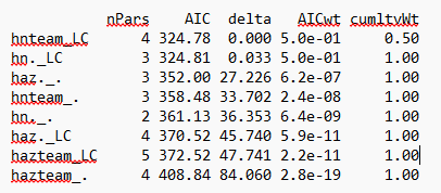
ModSelect
nPars AIC delta AICwt cumltvWt
hnLC_. 3 271.39 0.00 9.8e-01 0.98
hazLC_. 4 279.16 7.77 2.0e-02 1.00
hnLC_Team 4 324.78 53.39 2.5e-12 1.00
haz.. 3 352.00 80.61 3.1e-18 1.00
hn.
. 2 361.13 89.74 3.2e-20 1.00
hn._Team 3 363.11 91.72 1.2e-20 1.00
haz._Team 4 408.82 137.43 1.4e-30 1.00
hazLC_Team 5 410.82 139.43 5.2e-31 1.00

Due to the smaller AIC value, hnLC_Team would be the best-fit model to explain the result of the landcover and team covariate analysis.

ESHW9
1.523077 with absolute error < 8.6e-07

ESHW10
113.0809 with absolute error < 6e-07

hnLC_Team # show model output
Call:
distsamp(formula = ~Team ~ Landcover, data = TruncUMF, keyfun = “halfnorm”,
output = “density”, unitsOut = “ha”)

Density:
Estimate SE z P(>|z|)
(Intercept) -2.38 0.128 -18.7 7.86e-78
LandcoverWetland -1.04 0.179 -5.8 6.57e-09

Detection:
Estimate SE z P(>|z|)
(Intercept) 4.502 0.112 40.30 0.000
TeamB 0.195 0.135 1.44 0.149
AIC: 324.777

hazLC_Team # show model output

Call:
distsamp(formula = ~Landcover ~ Team, data = TruncUMF, keyfun = “hazard”,
output = “density”, unitsOut = “ha”)

Density:
Estimate SE z P(>|z|)
(Intercept) -2.9895 0.127 -23.567 8.42e-123
TeamB -0.0218 0.171 -0.127 8.99e-01

Detection:
Estimate SE z P(>|z|)
(Intercept) -7.35 NaN NaN NaN
LandcoverWetland -9.47 300 -0.0315 0.975

Hazard-rate(scale):
Estimate SE z P(>|z|)
-12 0.649 -18.4 5.67e-76

AIC: 410.8178

Hypotheses

#1 Survey team affects detectability of water deer

#2 Landcover affects density of water deer

#3 Modelled with both half-normal and hazard detection functions

The model that is the best fit for the data is the global model (i.e a combination of both hypothesis 1 and 2) when detection is modelled by a half-normal curve, this is because this model has a delta of 0 and the lowest AIC. The model hn._LC is a strong competitor as it also has a low AIC and a delta close to 0 with 0.033. This suggests that whilst the data supports both hypotheses, there is stronger support for hypothesis 2, Landcover affects density of water deer.

Detectabilty:

The half-normal standard deviation for Team A is 90.2m, in contrast the half-normal standard deviation for Team B is 110m. Team B’s detectability is higher than Team A’s.

CI’s

DetTeamA_CI
0.025 0.975
72.48405 112.3094
DetTeamB_CI
0.025 0.975
88.93429 135.1803

ESHW

ESHWTeamA
111.4124 with absolute error < 1.2e-12
ESHWTeamB
131.2631 with absolute error < 1.5e-12
ESHWTeamA$value/220
[1] 0.5064199 Detection probability for Team A within 220m from the transect is 50.6%
ESHWTeamB$value/220
[1] 0.5966503 Detecttion probability for Team B within 220m from the transect is 59.7%

Density:
The density estimate for water in grassland is 0.09 water deer per hectare (or 9 per square kilometre). The density estimate for water deer in wetland is 0.03 water deer per hectare (or 3 per square kilometre). The density estimate of water deer in grassland is three times more than in wetland. This is strong evidence for hypothesis #2. This is further supported when we look at the confidence intervals of the two land cover classes, as they do not overlap.

DensGrass_CI
0.025 0.975
0.07195514 0.1186252
DensWet_CI
0.025 0.975
0.02395455 0.04480861

Challenge:

The confidence intervals for detectability of Team A and Team B do not overlap, suggesting no significant difference between the two groups. If this is true, why is it in model with the best fit?