Analysis with R: Assignment 3

Submit your assignment for the Using output module in a reply to this topic

Remember to include these six elements:

  1. Your research question :question:
  2. The answer :bulb: to your question
  3. AIC-based evidence :1234: to support your conclusion
  4. Density estimate(s) :dart: with confidence intervals
  5. A brief reflection :thinking: on your next step, challenge you solved, problem you still have or leap of understanding
  6. Give specific and useful feedback :thumbsup: to a coursemate

Remember that you can always ask for help or share a draft of your assignment in our course discussion area if you want assistance

Research Question: Does the Density and detectability of Lemur change with distance?
Null model: Density and detectability are constant across the site (ie. The same on all transects)
Alternate hypothesis- density and detectability vary with transect length (and/or environmental covariates).
• Estimated Lemur density: 17 Lemurs per square kilometer with a standard error of 0.0924…
• As the 95% confidence interval spans 1.56 to 1.92, the true density of Lemur might vary from 16 to 19 deer per square kilometer
• 68% of the observations were recorded within 11.5 m of the transect and 95% within 23m
• Before truncation: The effective half strip is 14.4m for the Lemur transect. The detection probability is 30%.
• Density was below 15% beyond 20m, below 10% beyond 25m, and at 9% at 30m. Could this be due to Lemur’s behavior? Are they more used to human interaction or detection equipment?
• As lemur detection drastically decreased beyond 30m, the distance was truncated to 30m.
• After truncation: Effective half strip was 15.6m determined from the hazard rate model. The detection probability was 52%.
• Based on the AIC value, the best-fit model to assess density and detection after data truncation was the hazard rate model, the details of which are shown below.
• Unable to explore the covariates, will do so if posting assignments is still allowed.

Model Values, Detection/Density Table after truncation

       nPars     AIC  delta   AICwt cumltvWt
haz...     3  995.72   0.00 8.3e-01     0.83
hn..       2  998.88   3.16 1.7e-01     1.00
unif..     1 1301.53 305.80 3.3e-67     1.00

Core-Length of the transect affects the density of the lemur
Forest influences detection of lemur
The hypothesis with the most support is
Forest affects detectability and Core_length affects density, with detection modelled by a hazard curve


Call:
distsamp(formula = ~Forest ~ CoreLength_m, data = LemUMF2, keyfun = "hazard", 
    output = "density", unitsOut = "ha")

Density:
             Estimate    SE     z  P(>|z|)
(Intercept)    -0.154 0.113 -1.37 1.72e-01
CoreLength_m    1.418 0.179  7.94 2.05e-15

Detection:
               Estimate     SE     z   P(>|z|)
(Intercept)       2.140 0.0930 23.02 2.71e-117
ForestAnkarafa    0.547 0.0755  7.24  4.54e-13

Hazard-rate(scale):
 Estimate   SE    z  P(>|z|)
     1.13 0.12 9.44 3.78e-21

AIC: 530.5242
  • The intercept for density is negative , density is less than one lemur per hectare
  • The intercept for detection is positive, this is the coefficient for detectability on Anabohazo forest.
  • The intercept for Ankarafa forest is positive but lower than that of Anabohazo forest. Detectability in Ankarafa forest is lower than in Anabohazo forest.
  • The estimated densities are 1.31 animals per hectare with 300m of the transect covered by forest , and 1.71 animals per hectare with 500m of the transect covered by the forest. There is no overlap with the confidence intervals.

Challenge

When I backtransform detectability this is what I get,

Backtransformed linear combination(s) of Detection estimate(s)

 Estimate   SE LinComb (Intercept) ForestAnkarafa
      8.5 0.79    2.14           1              0

Transformation: exp 
> DetectAnkarafa
Backtransformed linear combination(s) of Detection estimate(s)

 Estimate    SE LinComb (Intercept) ForestAnkarafa
     14.7 0.893    2.69           1              1

Transformation: exp 
  • The hazard rate standard deviation in Anabohazo is only 8.5m
  • In contrast, the hazard rate standard deviation in Ankarafa is 14.7m. This would mean detectability in Anakara is higher than in Anabahazo, hence contradicting with the model intercepts. Which is which?
    • If I run the confidence intervals for detection, there is no overlap
    0.025    0.975
 13.03648 16.54442

AnabohazoCI
    0.025    0.975
 7.085644 10.20083

  • Effective Strip Half Width is 10m for our lemur transects in Anabahazo, with a detection probability of 36%
  • Effective Strip Half Width is 17m for our lemur transects in Anakarofa, with a detection probability of 58%

  1. AIC-based evidence :1234: to support your conclusion, for example a model comparison table

Model selection based on AICc:

            K   AICc Delta_AICc AICcWt Cum.Wt      LL
hZ._lemCL_F 5 535.98       0.00   0.95   0.95 -260.26
hn._lemF_CL 4 541.77       5.80   0.05   1.00 -265.22
hZ._lemCL   4 600.16      64.18   0.00   1.00 -294.41
hZ._lemF    4 601.23      65.25   0.00   1.00 -294.95
hn._lemCL   3 602.70      66.72   0.00   1.00 -297.43
hn._lemF    3 607.93      71.95   0.00   1.00 -300.04
  • Selecting the model to use using the AICc output was confusing for me, because the both models with the lowest AICc are different, half normal and the hazard rate.

Hi Sau, it sounds like you’ve run through the right process for a dataset without covariates, and your results are plausible for the lemur dataset. My results are slightly different because I chose a different truncation distance to you

A couple of points of clarification:

When you’re comparing covariate-free models, you’re simply asking which detection function is the best fit to the data. In this case, your null hypothesis is that the Uniform detection function is the best fit, because this assumes that detectability remains the same regardless of distance from the transect line[1]. It is also the model with the fewest parameters

Density and detectability cannot vary with transect length. Surveys themselves cannot affect the density. The only mechanism I can think of that might cause detectability to vary with transect length is observer fatigue, which is a factor you should try design out of field work. In your own surveys, you could check for observer fatigue by comparing the number of sightings in the first and second halves of transects


  1. At least, the way the uniform detecation function is implemented in unmarked, which doesn’t allow a slope coefficient for detection, i.e. a declining straight line ↩︎

Trying to share my results for this assignment:

I worked with the lemur dataset to answer the following questions:
1 – An Increased % of core forest within the transect will decrease the detectability of lemurs.
2 - The less disturbed forest, Anabohazo Forest, will have more density of lemurs as there is less anthropogenic disturbance.
Checked the hypothesis for the half-normal and the hazard detection function.

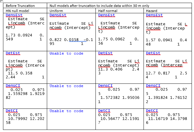
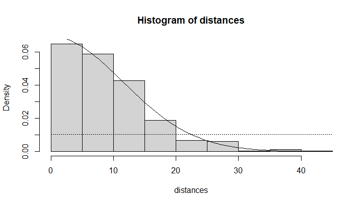
15% of the data fell within 22.5m, however I used 25m to truncate the dataset.
Results:
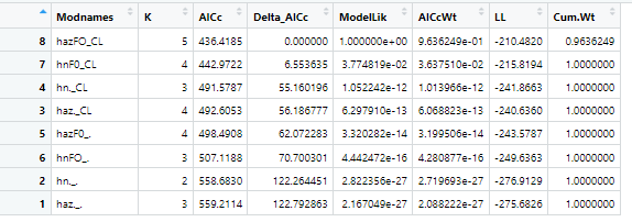
The results showed that the best model that fitted the data was the half normal detection function with Core percent and the Forest as covariates, as seen in the AICc table:
Model selection based on AICc:

  K   AICc Delta_AICc AICcWt Cum.Wt      LL
hnCO_FO 4 474.86       0.00   0.98   0.98 -231.76
hzCO_FO 5 482.67       7.81   0.02   1.00 -233.61
hz._FO  4 506.36      31.51   0.00   1.00 -247.51
hn._FO  3 506.44      31.58   0.00   1.00 -249.30
hnCO_.  3 588.71     113.86   0.00   1.00 -290.43
hzCO_.  4 594.80     119.95   0.00   1.00 -291.73
hz._.   3 609.83     134.97   0.00   1.00 -300.99
hn._.   2 610.40     135.55   0.00   1.00 -302.77

Best fit model:


hnCO_FO
Call:
distsamp(formula = ~CorePercent ~ Forest, data = lem_tru_UMF, 
    keyfun = "halfnorm", output = "density", unitsOut = "ha")


Density:
               Estimate     SE      z  P(>|z|)
(Intercept)       0.028 0.0871  0.321 7.48e-01
ForestAnkarafa    0.997 0.0963 10.355 3.99e-25


Detection:

            Estimate     SE     z   P(>|z|)
(Intercept)    1.978 0.0738 26.78 4.91e-158
CorePercent    0.788 0.1565  5.04  4.73e-07

AIC: 471.5221

Density estimates:
Anabohazo: 1.03 lemurs/ha; ranging from 0.87 lemurs/ha to 1.22 lemurs/ha
Ankarafa: 2.8 lemurs/ha; ranging from 2.45 lemurs/ha to 3.17 lemurs/ha
The more disturbed forest, Ankarafa, has rather higher density of lemurs than the less disturb forest.
Detectabiliity estimates:
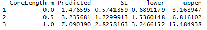
With 10% of core forest within the transect detectability rate is at 7.82m from the transect.
With a 60% of core forest within the transect detectability rate decreases to 11.6m.
Therefore our Null hyposthesis is true, an increased percentage of core forest within our transect decreases the detectability of the lemurs.
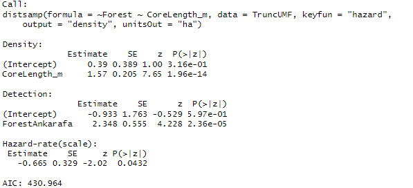
I wanted to go further to asses how good was the model used, however, I am stacked again.
How reliable is our model?
GOF

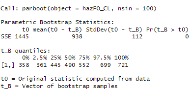
Call: parboot(object = hnCO_FO, nsim = 1000)

Parametric Bootstrap Statistics:
      t0 mean(t0 - t_B) StdDev(t0 - t_B) Pr(t_B > t0)
SSE 1436            950               98            0

t_B quantiles:
      0% 2.5% 25% 50% 75% 97.5% 100%
[1,] 244  327 414 478 548   690 1026

t0 = Original statistic computed from data
t_B = Vector of bootstrap samples

The p-value is 0 in this case, meaning that our model is a poor fit for this data.

I then calculated the estimated value of ^c to try and improve the model:

cHat estimate:
SSE
2.994418  

Seems there is a lack of independence of observations

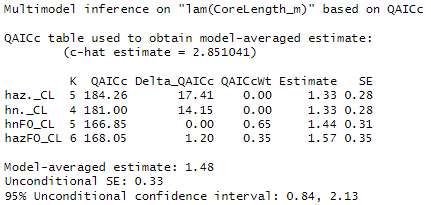
        K  QAICc Delta_QAICc QAICcWt Cum.Wt Quasi.LL
hnCO_FO 5 170.25        0.00    0.93   0.93   -77.40
hzCO_FO 6 176.43        6.18    0.04   0.97   -78.01
hn._FO  4 177.84        7.59    0.02   1.00   -83.25
hz._FO  5 180.77       10.52    0.00   1.00   -82.66
hnCO_.  4 205.32       35.07    0.00   1.00   -96.99
hn._.   3 210.07       39.82    0.00   1.00  -101.11
hzCO_.  5 210.31       40.06    0.00   1.00   -97.43
hz._.   4 212.37       42.12    0.00   1.00  -100.52
SumWt_Forest <- importance(models,
                        c.hat = cHat,
                        parm = "Forest",
                        parm.type= "lambda", 
                        second.order = TRUE) 

Importance values of 'lam(ForestAnkarafa)':
w+ (models including parameter): 1 
w- (models excluding parameter): 0

And I got a bit confused on the conclusions of these steps. Because the Sum of weights seems to say that the forest type has an influence on density. However, when using the expand.grid() function for predicting for multiple covariates, shows that none of the covariates has an effect. Not sure I am interpreting this right…

Below the code and results I got.

CI_dens
 			         0.025     0.975
lam(Int)           		  -0.1427598 0.1986864
lam(ForestAnkarafa)    0.8081677 1.1855487

CIDetect
  				 0.025      0.975
p(Int)      		   1.8330838    2.122539
p(CorePercent) 	   0.4815181    1.094935


predictionsFO <- cbind(
  ForestDF,
  predict(
    hnCO_FO,
    newdata = ForestDF,
    type="state"))
predictionsFO

Forest Predicted         SE     lower    upper
1 Anabohazo  1.028358 0.08957533 0.8669623 1.219799
2  Ankarafa  2.786598 0.18336074 2.4494268 3.170182

core_percent <- data.frame(
  CorePercent = c(0, 0.5, 1))

predictionsCO <- cbind(core_percent, 
                        predict(hnCO_FO,
                                newdata = core_percent,
                                type="det"))
predictionsCO

CorePercent Predicted        SE     lower     upper
1         0.0  7.226908 0.5336490  6.253140  8.352316
2         0.5 10.718001 0.4925153  9.794883 11.728119
3         1.0 15.895531 1.6682455 12.940198 19.525814

PredCO_FO <- cbind(cov_combinations,
                    round(
                      predict(hnCO_FO,
                              newdata = cov_combinations,
                              type="state")
                      , 3))
PredCO_FO
CorePercent    Forest Predicted    SE lower upper
1         0.00 Anabohazo     1.028 0.090 0.867  1.22
2         0.25 Anabohazo     1.028 0.090 0.867  1.22
3         0.50 Anabohazo     1.028 0.090 0.867  1.22
4         0.75 Anabohazo     1.028 0.090 0.867  1.22
5         1.00 Anabohazo     1.028 0.090 0.867  1.22
6         0.00  Ankarafa     2.787 0.183 2.449  3.17
7         0.25  Ankarafa     2.787 0.183 2.449  3.17
8         0.50  Ankarafa     2.787 0.183 2.449  3.17
9         0.75  Ankarafa     2.787 0.183 2.449  3.17
10        1.00  Ankarafa     2.787 0.183 2.449  3.17

Great work, @Nicorll ! Your results look sound, and your conclusions make sense.

Here are some questions and comments to check some details and refine your understanding and analytical process:

Transforming covariates

Did you transform your CoreLength_m covariate to bring it into a scale of c. zero to one, for example by converting it to kilometres?

Detectability between forests: Understanding hazard-rate coefficients

Unlike the half-normal detection function, the hazard-rate detection function does not have standard deviation as a parameter. Instead it has shape and scale. See here for a reminder

By including Forest as a predictor of detectability, you’re asking whether the shape of the hazard-rate detection function differs between Anabohazo and Ankarafa. Remember that the intercept represents the first category (Anabohazo = 2.14), and the coefficient for any category after the first must be added to the intercept to get the value for that category (Ankarafa = 2.14 + 0.55 = 2.69). So because Ankarafa has a positive coefficient, it has higher detectability than Anabohazo

Specifically, detectability in Anabohazo drops off closer to the transect (smaller shoulder), afterwards declining more slowly than in Ankarafa. Your backtransform() results, confidence intervals and ESHW/detection probability calculations confirm that detectability is lower in Anabohazo than in Ankarafa

Selecting the best model

Your top model has an AICc weight of 95%. This would be very strong evidence for that model provided the model set included a null model (like hz._.). Your model set doesn’t appear to contain a null model?

Your model names are a little confusing. Did your top model actually test for the effect of Core length on detectability, and the effect of Forest on density? Or is this just an error in the model names? Are the models which only include a single covariate holding the other variable (density or detectability) constant, i.e. the formula for hZ.lemF is ~Forest ~1?

Goodness of Fit test

What results did you Goodness of Fit test give you?

On the whole, I can see how hard you’ve worked, and it’s clear you’ve grasped the main points, apart from the apparent lack of a null model which it’s vital that you include in order to trust your covariate results

Well done, @Nuria - you’ve worked through the process, and correctly interpreted the results to choose your best model, and calculate densities. Great work! :muscle:

A few notes to help you grasp the last details on detectability and covariates:

Interpreting and calculating detectability

Be aware that predicted detectability is a probability, but when you back-transform your covariate coefficients for detectability, you are calculating the parameters of the detection function, not detectability directly. You need to calculate ESHW for a given core forest value, and combine that ESHW with your truncation distance to estimate detectability for that core forest value. I’ve included a worked example below

The positive coefficient for the effect of core forest on detectability tells us that they are positively related. In other words, detectability is higher on transects with a greater percentage of core forest. So the interpretation of these results:

is rather that:

  • In 10% core forest, detectability drops off more rapidly - 95% of lemurs were spotted within 15.6m (= 2 x 7.8m)
  • In 60% core forest. detectability extends further - 95% of lemurs were spotted within 23.2m

To calculate detection probability, use your backtransformed values. For example:

DetParamCore10 <- backTransform(linearComb(hnCO_FO, coefficients = c(1, 0.1), type = "det")) # Back-transformed detection parameter on a transect with 10% core forest
ESHW10 <- integrate(gxhn, 0, TruncDist, sigma = DetParamCore10@estimate) # Half-width in 10% core forest
DetProb10 <- ESHW10$value / TruncDist # Detectability in 10% core forest

When I do this, I get detection probabilities of:

  • 45% in 10% core forest
  • 69% in 60% core forest

Your exact answers will vary slightly as I used a different truncation distance, but they should be similar

Effect of covariates

When you say:

what information are you using to draw the conclusion that none of the covariates has an effect?

I can see that your 95% confidence intervals don’t overlap for the two forests, or for your chosen (widely-spaced) core forest percentages, and the CIs don’t include zero, which suggests that both covariates are meaningful predictors[1]

Given that your best model only includes Forest as a predictor of density[2], you only need to include Forest when calculating predicted density. Core percent won’t affect your density predictions because you didn’t include it as a predictor of density in your best model. Likewise for Forest: it won’t influence detectability in an expandgrid() matrix because it’s not a predictor of detectability in your best model

I hope that’s useful, and well done for persisting on the course!


  1. setting aside the GoF results, which suggest that we’re missing something fundamental in our analysis ↩︎

  2. Again, temporarily setting aside that our GoF testing suggests none of our models are adequate ↩︎

1 Like

Research Question

The density of lemurs is affected by core length in a transect and detectability is affected by forest fragmentation (Ankarafa or Anabohazo). Modelled at half-normal and hazard rate detection functions.

From the model selection table (w/ small correction factor) above we can see that model that most supports our hypotheses is the global model (density and detectability together) modelled with a hazard rate detection function. Output below:

Density estimates at different core lengths w/ confidence intervals.

predictionsCL

The above output shows that as the length of forest core on a transect increases them the density of lemurs increase also. The confidence intervals overlap with one another except for when core length is 0m and 1000m. Given that transect with the longest core length was 829m, we can say that core length does not have a biological meaningful effect on density.

Detectability estimates of the two forests w/ confidence intervals. (Ankarafa = fragmented, Anabohazo = not fragmented)

predictionsFO

From the estimates above and the negative intercept from the model output we can see that detectability Anabohazo forest is lower than in Ankarafa. Once again, the confidence intervals overlap, which means there is no meaningful difference between detectability between the two forests.

Whilst the hazFO_CL model was the strongest of all the models, it still hasn’t given us any evidence to support our hypotheses. Suggesting that in actuality the model fits our data poorly. There are various ways we can test for this. Firstly, a goodness of fit (GOF) test:

The p-value of the GOF test is below 0.05, which is significant. As our strongest model was the global model we cannot trust any of analysis given by out models. Secondly we can calculate the c^:

 SSE 

2.851041

A figure of 2.85 for the c^ means there is a lack of independence in our data.

Based on these two results it is likely that the two covariates of little importance were chosen for this analysis. To determine the importance of a particular covariate we can calculate summed weights of all the models that include that covariate.

Importance values of ‘lam(CoreLength_m)’:

w+ (models including parameter): 1
w- (models excluding parameter): 0

The summed weight of the models that include core length equals 1. This means that the covariate is a useful predictor of density, however this contradicts our analysis. The summed weight of the forest covariate = 0.99935. This indicates that ‘forest’ is a useful predictor for detectability. As we are still unsure whether our chosen covariates are important we can use evidence ratios.

Evidence ratio between models ‘hazFO_CL’ and ‘hazFO_.’:

Evidence ratio between models ‘haz.CL’ and 'haz..’:
27777.11

The results show that forest is not an important covariate as the evidence ratio is 0. The evidence ratio for core length is 27777.11 this means that models with core length as a covariate are 27777.11 times more likely than models that omit it. The below output shows the model-averaged parameter of all models that included core length.

Conclusion

The models were a bad fit for our data. But there was a useful take away that core length does impact density to some degree, however I’m not sure what that is. Hypotheses should be reassessed and different covariates considered in a new analysis.

Challenges

Evaluating the covariates seems to make things more confusing. :face_with_diagonal_mouth:

The model was a poor fit for the data, but one of my covariates was important according to the evidence ratios. But models with a supposed “unimportant” covariate are ranked higher in the AIC tables?

Unsure how to interpret the ModAvg table.